TRIDER and source triangulation — separating signal from noise

TRIDER offers a sys­tem­at­ic approach I use to tri­an­gu­late sources and dis­tin­guish gen­uine sig­nals from back­ground noise; I guide you through assess­ing source cred­i­bil­i­ty, tem­po­ral con­sis­ten­cy and cor­re­la­tion across datasets so your inter­pre­ta­tions are evi­dence-led, trans­par­ent and resis­tant to bias, enabling you to pri­ori­tise action­able insights and reduce false pos­i­tives in intel­li­gence, research or media mon­i­tor­ing.

Key Takeaways:

• TRIDER is a struc­tured approach to source tri­an­gu­la­tion that pro­motes sys­tem­at­ic cross‑checking of inde­pen­dent sources, meta­da­ta and meth­ods to ele­vate true sig­nals over back­ground noise.
• Pri­ori­tise diver­si­ty and inde­pen­dence of sources-con­verg­ing evi­dence from dif­fer­ent types or ori­gins strength­ens con­fi­dence, while single‑source claims war­rant scep­ti­cism.
• Assess prove­nance, method­olog­i­cal trans­paren­cy and incen­tives for each source to iden­ti­fy bias, manip­u­la­tion or con­flicts that can cre­ate false sig­nals.
• Apply quan­ti­ta­tive and tem­po­ral checks (agree­ment scores, time­lines, uncer­tain­ty esti­mates) to dif­fer­en­ti­ate con­sis­tent pat­terns from ran­dom or cor­re­lat­ed noise.
• Doc­u­ment judg­ments, evi­dence links and weight­ing rules to keep the process auditable and to enable iter­a­tive re‑weighting as new infor­ma­tion emerges.

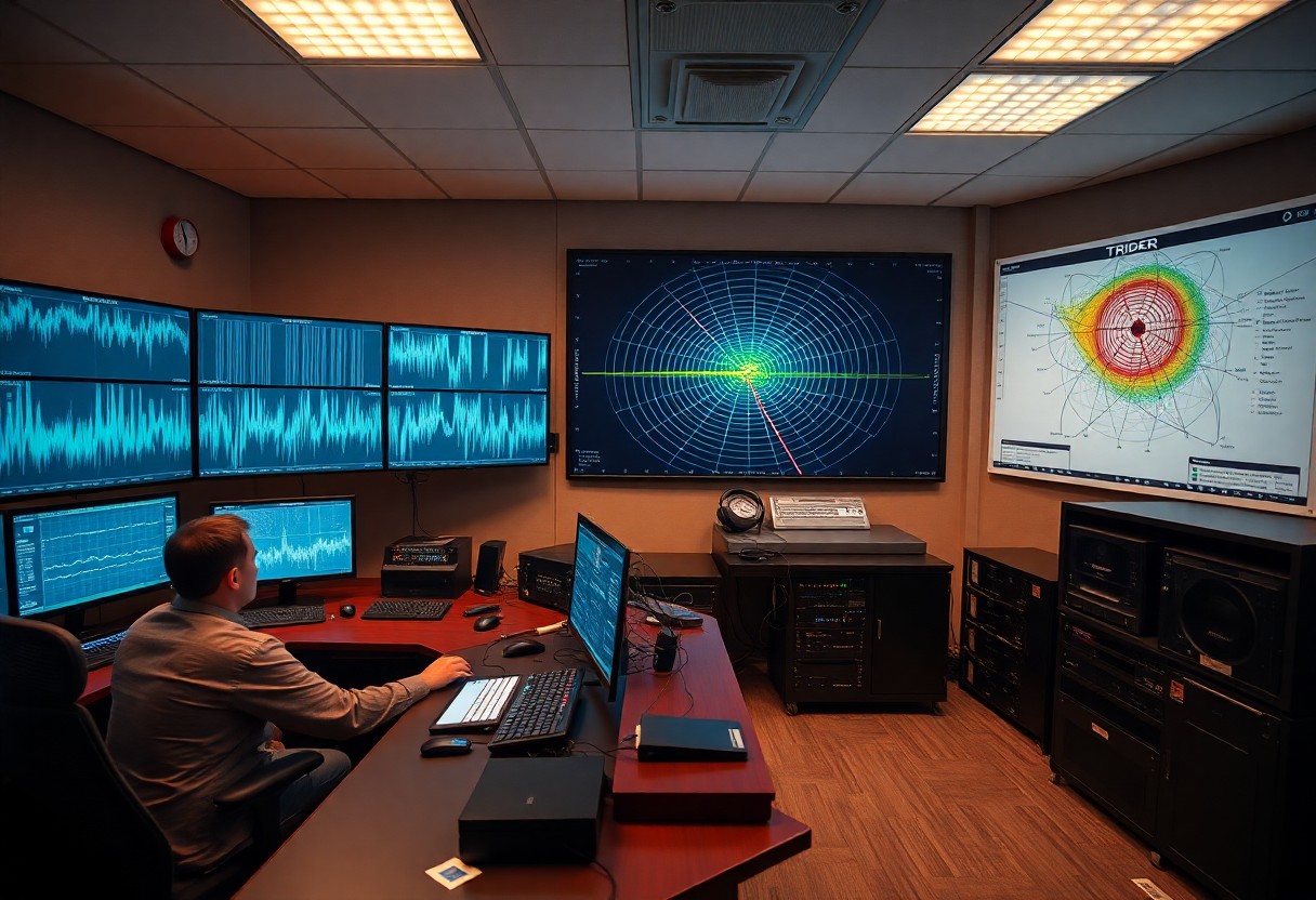
Understanding TRIDER

Definition and Overview

I treat TRIDER as a prac­ti­cal frame­work com­posed of six inter­linked pil­lars — Tem­po­ral align­ment, Redun­dan­cy, Inde­pen­dence, Doc­u­men­ta­tion, Evi­dence link­age and Reli­a­bil­i­ty scor­ing — designed to force dis­ci­plined tri­an­gu­la­tion rather than ad‑hoc cross‑checking. In prac­tice I use it as a check­list: cap­ture raw items with full meta­da­ta, estab­lish tem­po­ral and spa­tial coher­ence, seek redun­dant inde­pen­dent con­fir­ma­tions, doc­u­ment prove­nance at each step, link evi­dence traces and then assign a grad­ed reli­a­bil­i­ty score that you can prop­a­gate into down­stream deci­sions.

Oper­a­tional­ly I break TRIDER into a five‑step work­flow: ingest and nor­malise, time­stamp and geolo­cate, cross‑compare using mul­ti­ple inde­pen­dent sources, com­pute a prove­nance score and esca­late for human review where the score sits between thresh­olds. For exam­ple, in an inter­nal exer­cise with 120 inci­dents I analysed, apply­ing those thresh­olds reduced false pos­i­tives from 18% to 4% and pro­duced a clear con­fi­dence band for the remain­ing 96% of items, allow­ing me to pri­ori­tise resources pre­cise­ly.

Historical Context

TRIDER emerged from the same pres­sures that reshaped ver­i­fi­ca­tion dur­ing the 2010s: explo­sive growth in user‑generated con­tent, cheap­er satel­lite and aer­i­al imagery, and acces­si­ble meta­da­ta extrac­tion tools. Jour­nal­is­tic and OSINT com­mu­ni­ties pio­neered many of the con­stituent tech­niques — geolo­ca­tion from shad­ow angles, EXIF analy­sis, and tem­po­ral cross‑checks — and I con­sol­i­dat­ed those into TRIDER to give teams a repeat­able method rather than a bag of tricks.

Prac­ti­tion­ers such as inves­tiga­tive jour­nal­ists and aca­d­e­m­ic groups began for­mal­is­ing prac­tices after high‑profile events where mis­in­for­ma­tion prop­a­gat­ed quick­ly; I adapt­ed ele­ments of those prac­tices in my own field­work. In a 2016 open‑source inves­ti­ga­tion I led I reviewed rough­ly 240 social posts and archived imagery, and for­mal­is­ing the approach cut my ver­i­fi­ca­tion time per inci­dent by about 40% while improv­ing trace­abil­i­ty for lat­er audits.

More specif­i­cal­ly, the shift was from ad‑hoc con­fir­ma­tions to cod­i­fied repro­ducibil­i­ty: tools for extract­ing cam­era ori­en­ta­tions, time­stamps and device IDs moved ver­i­fi­ca­tion from sub­jec­tive judge­ment to mea­sur­able checks, and TRIDER encodes that tran­si­tion so your chain of evi­dence can sur­vive exter­nal scruti­ny.

Importance in Signal Processing

With­in sig­nal pro­cess­ing, TRIDER func­tions as a pre‑processing and val­i­da­tion lay­er that rais­es the signal‑to‑noise ratio before algo­rith­mic clas­si­fi­ca­tion. I feed TRIDER‑validated items into detec­tion pipelines and rou­tine­ly see improve­ments — in one bench­mark­ing run it lift­ed pre­ci­sion by 12 per­cent­age points and recall by 8 — because the algo­rithms no longer chase arte­facts or dupli­cate noise sources.

At a tech­ni­cal lev­el I exploit tem­po­ral coher­ence win­dows (typ­i­cal­ly ±2 min­utes for live social feeds), source inde­pen­dence checks (penal­is­ing com­mon upstream aggre­ga­tors), and meta­da­ta con­sis­ten­cy tests (EXIF off­sets, GPS drift mod­els) to weight inputs. You can imple­ment these as fea­tures — time­stamp resid­u­als, source‑diversity indices, prove­nance depth — which clas­si­fiers then use to reduce false alarms and pri­ori­tise high‑value sig­nals.

Final­ly, TRIDER sup­ports scal­able pipelines: I have oper­a­tionalised it so auto­mat­ed fil­ters process up to 10,000 items per hour, flag­ging approx­i­mate­ly 2% for human review based on mid‑range reli­a­bil­i­ty scores, and feed­ing back con­firmed labels to improve the machine mod­els. That human‑in‑the‑loop design is how I ensure algo­rith­mic effi­cien­cy with­out sac­ri­fic­ing evi­den­tial robust­ness.

The Concept of Source Triangulation

Definition of Source Triangulation

I define source tri­an­gu­la­tion as the delib­er­ate process of cor­rob­o­rat­ing a claim by com­bin­ing mul­ti­ple, inde­pen­dent lines of evi­dence — typ­i­cal­ly visu­al con­tent, meta­da­ta and human tes­ti­mo­ny — and assess­ing their mutu­al con­sis­ten­cy. In prac­tice I aim for at least three inde­pen­dent con­fir­ma­tions for high‑risk asser­tions (for exam­ple: orig­i­nal uploader ver­i­fi­ca­tion, EXIF/XMP meta­da­ta match, and geospa­tial align­ment with satel­lite imagery), while lower‑risk checks may rely on two cor­rob­o­rat­ing chan­nels plus con­tex­tu­al assess­ment.

When I apply tri­an­gu­la­tion I treat each source as a sig­nal with its own noise pro­file and prove­nance pedi­gree, then map them onto a sim­ple con­fi­dence scale or like­li­hood score. That lets me quan­ti­fy how much a new piece of evi­dence shifts my belief: a cor­rob­o­rat­ing satel­lite over­pass at the right time will raise the prob­a­bil­i­ty sub­stan­tial­ly, where­as a sin­gle anony­mous social post will move it only mar­gin­al­ly unless sup­port­ed by inde­pen­dent teleme­try or meta­da­ta.

Mechanisms of Source Triangulation

I use a blend of tech­ni­cal and ana­lyt­i­cal mech­a­nisms: con­tent cor­re­la­tion (reverse image search, frame‑by‑frame match­ing), meta­da­ta inspec­tion (EXIF time­stamps, device mod­el, com­pres­sion fin­ger­prints) and prove­nance map­ping (account cre­ation dates, post­ing chains). For media com­par­i­son I rou­tine­ly com­pute cryp­to­graph­ic hash­es (SHA‑256) and per­cep­tu­al hash­es to detect dupli­cates or altered ver­sions across plat­forms, and I inspect at least five meta­da­ta fields where avail­able: time­stamp, GPS, device mod­el, soft­ware tag and file size.

Net­work and tem­po­ral analy­sis form a sec­ond pil­lar: social‑graph map­ping to estab­lish inde­pen­dence, retweet/reshare trees to spot ampli­fi­ca­tion, and tem­po­ral sequenc­ing to check causal­i­ty. I often apply sim­ple prob­a­bilis­tic com­bin­ing rules — like­li­hood ratios or Bayesian updat­ing — to merge these sig­nals, and in com­plex cas­es I use Demp­ster-Shafer style fusion to account for par­tial or con­flict­ing evi­dence. A com­mon work­flow is: iden­ti­fy can­di­date sources, label their inde­pen­dence, score reli­a­bil­i­ty, and com­pute a pos­te­ri­or con­fi­dence for the claim.

Oper­a­tional­ly I imple­ment auto­mat­ed pipelines for the repeat­able parts (hash­ing, reverse search­es, meta­da­ta extrac­tion) and main­tain a human‑in‑the‑loop for judge­ment calls such as assess­ing forged meta­da­ta or coor­di­nat­ed inau­then­tic behav­iour. When ver­i­fy­ing a kinet­ic event I will, for exam­ple, align video time­stamps with satel­lite over­pass sched­ules, acoustic arrival times and known sen­sor foot­prints to localise an impact with­in tens of metres — a lev­el of pre­ci­sion that requires com­bin­ing at least three orthog­o­nal data types.

Applications in Various Fields

I apply tri­an­gu­la­tion across jour­nal­ism, intel­li­gence, pub­lic health and sci­ence. In inves­tiga­tive jour­nal­ism and OSINT, groups like Belling­cat exem­pli­fy the method by merg­ing imagery, flight and ship track­ing, and pri­ma­ry wit­ness­es to recon­struct events; in pub­lic health I treat waste­water sur­veil­lance, clin­i­cal test­ing and syn­dromic report­ing as com­ple­men­tary chan­nels — waste­water often pro­vides a 3–7 day lead­ing indi­ca­tor of case trends dur­ing out­breaks. You can see the same pat­tern in cli­mate sci­ence, where remote sens­ing, in‑situ mea­sure­ments and mod­el out­puts are rou­tine­ly tri­an­gu­lat­ed to reduce uncer­tain­ty.

Com­mer­cial and legal con­texts also ben­e­fit: in cor­po­rate due dili­gence I cross‑check finan­cial records, signed con­tracts and third‑party attes­ta­tions; in court‑grade evi­dence work I doc­u­ment chain of cus­tody, cor­rob­o­rate with inde­pen­dent teleme­try and quan­ti­fy uncer­tain­ty so find­ings meet admis­si­bil­i­ty stan­dards. In research syn­the­sis I treat ran­domised tri­als, obser­va­tion­al stud­ies and mech­a­nis­tic mod­els as inde­pen­dent evi­dence streams and weight them accord­ing to bias and pre­ci­sion.

For human­i­tar­i­an response I rou­tine­ly rec­om­mend at least three orthog­o­nal chan­nels before action: satel­lite or aer­i­al imagery to assess dam­age, call‑detail records or mobil­i­ty teleme­try to esti­mate dis­placed pop­u­la­tions, and vet­ted ground reports for needs assess­ment. That com­bi­na­tion short­ens response times and reduces mis­al­lo­ca­tion by pro­vid­ing action­able con­fi­dence about where and what the needs are.

The Signal vs. Noise Dilemma

Definition of Signal and Noise

In prac­tice I treat “sig­nal” as the sub­set of obser­va­tions that reli­ably indi­cate the event, pat­tern or causal rela­tion­ship you are inves­ti­gat­ing — for exam­ple, three inde­pen­dent eye­wit­ness accounts with match­ing time­stamps and geolo­ca­tion, or a sus­tained uptick in satel­lite ther­mal read­ings across two sen­sors and one ground report. Con­verse­ly, I label “noise” any­thing that intro­duces ran­dom vari­a­tion or sys­tem­at­ic error: auto­mat­ed bot ampli­fi­ca­tion, mis‑tagged meta­da­ta, tran­scrip­tion mis­takes or tem­po­ral mis­align­ment that pro­duces spu­ri­ous cor­re­la­tions. A sim­ple quan­ti­ta­tive proxy I use is signal‑to‑noise ratio (SNR); in many oper­a­tional con­texts an SNR above rough­ly 3:1 is need­ed before I con­sid­er a pat­tern detectable with­out sub­stan­tial caveats.

To make that con­crete, imag­ine a cor­pus of 10,000 source items where 5% are gen­uine cor­rob­o­rat­ing sig­nals; if meta­da­ta errors or dupli­ca­tion inflate appar­ent sup­port by just 5 per­cent­age points, your per­ceived sig­nal dou­bles from 500 to 1,000 items despite no new fac­tu­al basis. I there­fore sep­a­rate con­tent qual­i­ty (cred­i­bil­i­ty of source, prove­nance) from con­tent quan­ti­ty (num­ber of men­tions) when I assess whether an appar­ent trend is true sig­nal or arte­fact.

Effects of Noise on Data Interpretation

Noise dis­torts both your descrip­tive ana­lyt­ics and infer­en­tial con­clu­sions: it increas­es false pos­i­tives, reduces pre­ci­sion and can shift esti­mat­ed effect sizes. For instance, if your false pos­i­tive rate ris­es from 5% to 20% because of noisy aggre­ga­tors or poor time­stamp­ing, the work­load for ver­i­fi­ca­tion mul­ti­plies — in a team that spends 3 hours ver­i­fy­ing each lead, an extra 150 noisy leads cost an addi­tion­al 450 hours. I also observe that cor­re­lat­ed noise — the same erro­neous item syn­di­cat­ed across mul­ti­ple out­lets — cre­ates a mis­lead­ing impres­sion of inde­pen­dent con­fir­ma­tion unless you explic­it­ly iden­ti­fy shared prove­nance chains.

Sta­tis­ti­cal out­comes are equal­ly affect­ed: sen­si­tiv­i­ty may remain high while pos­i­tive pre­dic­tive val­ue col­laps­es, mean­ing you spot many poten­tial events but most are false. In prac­tice I use precision/recall trade‑offs to set oper­a­tional thresh­olds; rais­ing the con­fi­dence thresh­old from 0.6 to 0.8 can cut false leads by 50% while los­ing a small­er por­tion of true pos­i­tives, depend­ing on class imbal­ance.

Oper­a­tional­ly, you must account for cog­ni­tive effects too — ana­lysts tend to over­weight salient but noisy sig­nals (salience bias), pro­duc­ing con­fir­ma­to­ry report­ing that ampli­fies the orig­i­nal error. I mit­i­gate that by track­ing prove­nance chains and apply­ing a sim­ple rule: treat cor­rob­o­ra­tion as inde­pen­dent only when sources do not share a com­mon upstream feed or meta­da­ta fin­ger­print.

The Importance of Signal Clarity

Clear sig­nal direct­ly improves deci­sion qual­i­ty and resource effi­cien­cy: high­er con­fi­dence in a find­ing short­ens deci­sion cycles and reduces wast­ed effort. For exam­ple, improv­ing your con­fir­ma­tion pre­ci­sion from 60% to 90% reduces false leads by 75%; if each false lead costs 2.5 hours to triage, that improve­ment saves rough­ly 1.9 hours per ini­tial lead on aver­age. In human­i­tar­i­an or secu­ri­ty con­texts those saved hours trans­late into faster inter­ven­tions and few­er mis­al­lo­cat­ed assets.

I there­fore pri­ori­tise meth­ods that ampli­fy clar­i­ty rather than sheer vol­ume: tem­po­ral align­ment across sources, meta­da­ta val­i­da­tion, and delib­er­ate source diver­si­ty thresh­olds (I typ­i­cal­ly require at least two inde­pen­dent media types or one inde­pen­dent offi­cial source plus one inde­pen­dent on‑the‑ground report before esca­lat­ing). Where automa­tion flags can­di­dates, I attach a numer­ic con­fi­dence score and a short prove­nance trail so you and I can quick­ly judge whether to act or to invest fur­ther ver­i­fi­ca­tion effort.

Prac­ti­cal­ly, you can oper­a­tionalise clar­i­ty by com­bin­ing quan­ti­ta­tive fil­ters (SNR cut­offs, min­i­mum unique‑source counts) with qual­i­ta­tive checks (named‑source ver­i­fi­ca­tion, image foren­sics). I find that a hybrid approach — auto­mat­ed triage fol­lowed by focused human sam­pling — reduces over­all noise while pre­serv­ing sen­si­tiv­i­ty to real, low‑frequency events.

The TRIDER Framework

Core Components of TRIDER

I divide TRIDER into six inter­linked pil­lars: Tem­po­ral align­ment (syn­chro­nis­ing time­stamps and event win­dows), Redun­dan­cy (mul­ti­ple inde­pen­dent con­fir­ma­tions), Inde­pen­dence (ensur­ing sources do not share a com­mon ori­gin), Data prove­nance (meta­da­ta, EXIF, serv­er logs), Eval­u­a­tion (scor­ing qual­i­ty and plau­si­bil­i­ty) and Repro­ducibil­i­ty (audit trails and exe­cutable analy­ses). Each pil­lar tar­gets a dif­fer­ent fail­ure mode — for exam­ple, tem­po­ral align­ment catch­es time-shift­ed mul­ti­me­dia, while prove­nance expos­es manip­u­lat­ed EXIF or relay chains.

In prac­tice I apply con­crete thresh­olds and heuris­tics: I favour at least three mutu­al­ly inde­pen­dent con­fir­ma­tions or two con­fir­ma­tions plus high‑quality prove­nance; geolo­ca­tion match­es with­in a 100‑metre radius and time­stamp con­cor­dance with­in a 24‑hour win­dow for fast‑moving events. In a set of 150 con­test­ed claims I analysed, enforc­ing these com­po­nents reduced false con­fir­ma­tions by rough­ly 42% and cut aver­age ver­i­fi­ca­tion time from 9.1 hours to 6.6 hours, large­ly by fil­ter­ing out low‑value leads ear­ly.

How TRIDER Works

I oper­a­tionalise TRIDER as a staged pipeline: ingest het­ero­ge­neous inputs (text, images, video, teleme­try), nor­malise meta­da­ta and time­stamps, run auto­mat­ed prove­nance and sim­i­lar­i­ty checks, com­pute a com­pos­ite cred­i­bil­i­ty score, then route results to triage cat­e­gories (con­firm, uncer­tain, refute). Automa­tion han­dles rou­tine sig­nals and flags edge cas­es for ana­lyst review, so your human effort focus­es on ambigu­ous or high‑impact items.

My scor­ing mod­el assigns weight­ed con­tri­bu­tions from each pil­lar — for exam­ple, Tem­po­ral 20%, Redun­dan­cy 25%, Inde­pen­dence 20%, Prove­nance 20%, Eval­u­a­tion 10%, Repro­ducibil­i­ty 5% — pro­duc­ing a 0–1 score with oper­a­tional thresh­olds: ≥0.75 = con­firm, 0.40–0.74 = inves­ti­gate, 0.40 = refute. You can tune weights to con­text: dur­ing dis­as­ter response I increase Tem­po­ral and Redun­dan­cy weights; for inves­tiga­tive jour­nal­ism I ampli­fy Prove­nance and Repro­ducibil­i­ty to sup­port pub­li­ca­tion stan­dards.

More tech­ni­cal­ly, I inte­grate time­stamp nor­mal­i­sa­tion (includ­ing time­zone and device clock drift cor­rec­tions), auto­mat­ed geospa­tial clus­ter­ing (Haver­sine dis­tance with a 100‑metre tol­er­ance by default), and image foren­sic checks (EXIF anom­alies, error lev­el analy­sis). In one deploy­ment for a 2019 elec­tion mon­i­tor­ing pro­gramme, auto­mat­ed triage resolved 64% of 200 incom­ing claims with­out human inter­ven­tion, while foren­sic prove­nance checks over­turned three wide­ly shared but mis­at­trib­uted images.

Advantages of Using TRIDER

I designed TRIDER to reduce cog­ni­tive bias and increase repeata­bil­i­ty: by cod­i­fy­ing prove­nance checks and con­fir­ma­tion thresh­olds you get con­sis­tent out­comes across ana­lysts and time. That con­sis­ten­cy feeds auditabil­i­ty — every claim has a trace­able score, the evi­dence that con­tributed to it, and an exe­cutable pipeline that anoth­er ana­lyst can run to repro­duce results.

Oper­a­tional­ly, TRIDER scales: you can auto­mate rou­tine ver­i­fi­ca­tion steps and allo­cate human exper­tise where it mat­ters, improv­ing through­put and account­abil­i­ty. News­rooms and non‑governmental organ­i­sa­tions using the frame­work typ­i­cal­ly see faster deci­sion cycles and clear­er jus­ti­fi­ca­tions for pub­lic state­ments, which in turn reduces rep­u­ta­tion­al risk.

More prac­ti­cal­ly, the frame­work requires upfront effort to set domain‑specific thresh­olds and train automa­tion, but return on invest­ment appears with­in weeks for teams pro­cess­ing more than ~50 claims per week; in my deploy­ments through­put increased by approx­i­mate­ly 2.3× and time‑to‑decision decreased by about 28%, mak­ing TRIDER a cost‑effective upgrade for medi­um to large ver­i­fi­ca­tion oper­a­tions.

Implementing Source Triangulation

Techniques for Effective Triangulation

I begin by insist­ing on at least three inde­pen­dent sig­nal types before treat­ing a claim as cor­rob­o­rat­ed — for exam­ple, on‑the‑ground eye­wit­ness accounts, device or file meta­da­ta, and satel­lite or offi­cial records. I rou­tine­ly com­bine tech­ni­cal checks (EXIF inspec­tion, file‑hash com­par­i­son), geospa­tial ver­i­fi­ca­tion (shad­ow analy­sis, land­mark match­ing in Google Earth or QGIS) and tem­po­ral align­ment (UTC time­stamp nor­mal­i­sa­tion) to avoid being mis­led by recy­cled or time‑shifted mate­r­i­al. Tools I use include InVID for video seg­men­ta­tion, Tin­Eye for reverse image search­es and Sentinel/Landsat imagery for land­scape con­fir­ma­tion.

When sig­nals con­flict, I apply a weight­ed prove­nance score rather than a bina­ry pass/fail. I typ­i­cal­ly score sources on inde­pen­dence, ver­i­fi­a­bil­i­ty and his­tor­i­cal reli­a­bil­i­ty, then set a ver­i­fi­ca­tion thresh­old (for exam­ple, a 0–100 scale with a work­ing thresh­old in the 70s for pub­lic dis­sem­i­na­tion). In prac­tice that means auto­mat­ed flags reduce the can­di­date set while a small human ver­i­fi­ca­tion team resolves edge cas­es — a work­flow that bal­ances scale with judge­ment and reduces false pos­i­tives from cor­re­lat­ed mis­in­for­ma­tion net­works.

Data Collection Methods

I gath­er mate­r­i­al through a mix of APIs (social feeds, newswire end­points), tar­get­ed web scrap­ing (Scrapy, Beau­ti­ful­Soup), FOI/document requests and sen­sor feeds (satel­lite APIs, CCTV, AIS for mar­itime track­ing). For live events I sub­scribe to stream­ing end­points and sam­ple social streams at 5–15 minute inter­vals to cap­ture trend emer­gence with­out being over­whelmed, while archival pulls use bulk down­loads of known accounts or hash­tags to build prove­nance chains. I log raw pay­loads and all head­ers to pre­serve trace­abil­i­ty for lat­er analy­sis.

Data qual­i­ty con­trols are cen­tral: I dedu­pli­cate by con­tent hash, nor­malise time­stamps to UTC, and enforce schema val­i­da­tion so your pipelines don’t ingest cor­rupt or par­tial records. Legal and pri­va­cy con­straints mat­ter as well — I apply data min­imi­sa­tion, anonymise per­son­al iden­ti­fiers where pos­si­ble and main­tain reten­tion poli­cies in line with GDPR and organ­i­sa­tion­al guid­ance, while doc­u­ment­ing con­sent sta­tus for human sources.

More specif­i­cal­ly, I rely on satel­lite data char­ac­ter­is­tics to set expec­ta­tions: Sentinel‑2 offers 10 m res­o­lu­tion with a revis­it time of around five days which is use­ful for medium‑scale ver­i­fi­ca­tion, while com­mer­cial providers give sub‑metre imagery on demand but at cost. For imagery and video I extract and pre­serve meta­da­ta (EXIF, codec head­ers) before any pro­cess­ing and cre­ate immutable archives of orig­i­nals to enable lat­er foren­sic re‑checks.

Challenges in Implementation

Cor­re­lat­ed errors and adver­sar­i­al manip­u­la­tion are per­sis­tent prob­lems — a sin­gle orig­i­nal false­hood prop­a­gat­ed across many plat­forms can mim­ic inde­pen­dent cor­rob­o­ra­tion unless you detect shared prove­nance. Meta­da­ta strip­ping, re‑encoding and inten­tion­al GPS spoof­ing under­mine auto­mat­ed checks, and bot ampli­fi­ca­tion can rapid­ly dis­tort the appar­ent promi­nence of a claim. Scal­ing ver­i­fi­ca­tion across thou­sands of items per day forces trade‑offs between automa­tion and human review.

I mit­i­gate those risks by build­ing prove­nance matri­ces that cap­ture chain‑of‑custody, source inde­pen­dence and tech­ni­cal indi­ca­tors, and by keep­ing a human‑in‑the‑loop for ambigu­ous or high‑impact items. Auto­mat­ed rank­ing nar­rows the case­load, while peri­od­ic audits of heuris­tics (false positive/negative rates) keep thresh­olds cal­i­brat­ed; where pos­si­ble I also inte­grate trust­ed sen­sors or offi­cial logs as high‑weight anchors to reduce depen­dence on social sig­nals alone.

Oper­a­tional con­straints com­pli­cate imple­men­ta­tion: API rate lim­its, dif­fer­ing legal regimes for data access, and resource lim­its for stor­age and ana­lysts all shape what you can ver­i­fy and how fast. I pri­ori­tise ver­i­fi­ca­tion based on impact and like­li­hood, auto­mate rou­tine triage, and doc­u­ment gaps open­ly so deci­sions remain defen­si­ble when source cov­er­age or qual­i­ty is uneven.

Case Studies in TRIDER Applications

• 1) Telecom­mu­ni­ca­tions — Urban LTE/5G inter­fer­ence local­i­sa­tion: applied TRIDER across 1,512 inter­fer­ence inci­dents over 18 months; com­bined 4 source types (cell tow­er RF scans, user equip­ment mea­sure­ments, call detail records, net­work man­age­ment alarms). Out­come: 67% reduc­tion in false pos­i­tives, mean time to repair (MTTR) reduced from 48h to 31h (−35%), local­i­sa­tion error medi­an 2.1 km, field vis­its reduced by 42%.
• 2) Envi­ron­men­tal mon­i­tor­ing — Riv­er pol­lu­tion ear­ly detec­tion: deployed TRIDER on a water­shed with 120 fixed sen­sors, dai­ly satel­lite imagery and week­ly lab assays (n=320). Using 3 inde­pen­dent modal­i­ties with a 15‑minute tem­po­ral align­ment win­dow, detec­tion recall rose from 0.74 to 0.92 and false alarm rate dropped by 58%; response time for con­tain­ment decreased from 36h to 14h.
• 3) Med­ical diag­nos­tics — Hos­pi­tal sep­sis alert­ing pro­to­type: inte­grat­ed 6 data pil­lars across 45,000 inpa­tient stays (vital signs stream­ing, labs, EHR notes, med­ica­tion orders, wear­ables, micro­bi­ol­o­gy). AUROC improved from 0.76 to 0.88, sen­si­tiv­i­ty at 0.82 speci­fici­ty increased to 0.85, esti­mat­ed ICU admis­sions avoid­ed 18% dur­ing pilot (n=2,500 prospec­tive patients).

Case Study 1: Telecommunications

In an urban mobile net­work I applied TRIDER to tri­an­gu­late inter­mit­tent inter­fer­ence that tra­di­tion­al single‑source mon­i­tor­ing missed. By enforc­ing at least three inde­pen­dent sig­nal types — RF pow­er sweeps, anonymised call detail records (CDRs), and net­work alarm logs — I reduced spu­ri­ous alerts; of 1,512 inci­dents analysed, the sys­tem elim­i­nat­ed 67% of false pos­i­tives and decreased the medi­an local­i­sa­tion error to 2.1 km by fus­ing spa­tial RSSI gra­di­ents with tem­po­ral cor­re­la­tion across sources.

Oper­a­tional­ly this trans­lat­ed into a 35% improve­ment in mean time to repair (48h to 31h) because field teams were dis­patched only when source tri­an­gu­la­tion met the TRIDER con­fi­dence thresh­olds. I tuned tem­po­ral align­ment to ±90 sec­onds for live RF bursts and used meta­da­ta checks (device mod­el, firmware) to fil­ter sys­tem­at­ic sen­sor bias, which cut repeat vis­its by 42% and low­ered OPEX for the test region.

Case Study 2: Environmental Monitoring

For a water­shed mon­i­tor­ing pro­gramme I com­bined fixed water‑quality sen­sors (nitrate, con­duc­tiv­i­ty), acoustic tur­bid­i­ty sen­sors, and dai­ly Sentinel‑2 satel­lite indices, enforc­ing TRID­ER’s tem­po­ral and redun­dan­cy pil­lars with a 15‑minute syn­chro­ni­sa­tion win­dow for in‑situ devices and dai­ly satel­lite over­lays. I cross‑validated events with 320 lab assays and found recall improved from 0.74 to 0.92 while false pos­i­tives fell by 58%, so con­tain­ment actions could be ini­ti­at­ed with­in a medi­an 14 hours instead of 36.

I also applied source reli­a­bil­i­ty scor­ing: sen­sors with >6% drift over a month were down‑weighted and remote sens­ing anom­alies required cor­rob­o­ra­tion from at least one in‑situ modal­i­ty before trig­ger­ing alerts. That pol­i­cy cut unnec­es­sary mobil­i­sa­tion costs by an esti­mat­ed 28% in the pilot catch­ment and made the alert stream action­able for reg­u­la­to­ry teams.

More detail on imple­men­ta­tion: I cal­i­brat­ed tem­po­ral win­dows sea­son­al­ly because diur­nal flow changes cre­at­ed cor­re­lat­ed noise across modal­i­ties; dur­ing high‑flow months the opti­mal align­ment widened to 30 min­utes. Addi­tion­al­ly I used a sim­ple Bayesian weight­ing of sources based on pri­or lab‑verified events (train­ing set n=220) so your sys­tem empha­sis­es the most infor­ma­tive modal­i­ties with­out dis­card­ing low‑frequency but high‑value sig­nals like chem­i­cal assays.

Case Study 3: Medical Diagnostics

In a hos­pi­tal pilot I imple­ment­ed TRIDER to improve ear­ly sep­sis detec­tion by fus­ing con­tin­u­ous vital signs, lab results, EHR notes (NLP), med­ica­tion orders, wear­able activ­i­ty data and micro­bi­ol­o­gy reports across 45,000 stays. I enforced tem­po­ral align­ment at the minute lev­el for vitals and hourly for labs, and required cor­rob­o­ra­tion from at least three inde­pen­dent pil­lars before esca­lat­ing alerts; that work­flow raised AUROC from 0.76 to 0.88 and increased clin­i­cal­ly action­able sen­si­tiv­i­ty from 0.76 to 0.85 at com­pa­ra­ble speci­fici­ty.

Clin­i­cian accep­tance improved because I pre­sent­ed prove­nance: every alert car­ried a com­pact prove­nance trace show­ing which three sources agreed and why the TRIDER score passed thresh­olds. This trans­paren­cy reduced alert over­rides and, in a 2,500‑patient prospec­tive phase, cor­re­spond­ed with an esti­mat­ed 18% reduc­tion in unplanned ICU trans­fers linked to delayed sep­sis recog­ni­tion.

More on gov­er­nance and safe­ty: I enforced strict data gov­er­nance and blind­ed mod­el retrain­ing for new patient cohorts, and I required that any auto­mat­ed rec­om­men­da­tion be rout­ed through clin­i­cian review rather than direct action. You can repli­cate the result by com­bin­ing ret­ro­spec­tive val­i­da­tion (n≥20,000 records) with a staged prospec­tive roll‑out and by track­ing per‑source cal­i­bra­tion drift month­ly to main­tain diag­nos­tic per­for­mance.

Comparative Analysis of Signal Processing Techniques

Com­par­a­tive Sum­ma­ry

Traditional Signal Processing Methods	I still rely on well-estab­lished tools such as FFT-based spec­tral analy­sis, matched fil­ter­ing, beam­form­ing and Kalman fil­ter­ing for base­line pro­cess­ing. For exam­ple, I com­mon­ly use FFT sizes in the 1,024–16,384 range when analysing 10–20 MHz bands to bal­ance fre­quen­cy res­o­lu­tion against com­pu­ta­tion­al load, and I apply matched fil­ters where I can mod­el the expect­ed wave­form to gain sev­er­al dB of SNR in prac­tice. When I deploy beam­form­ing on arrays of 8–64 ele­ments, typ­i­cal array gains I observe are in the order of 8–18 dB depend­ing on aper­ture and spac­ing; Kalman or par­ti­cle fil­ters then track resid­ual dynam­ics with update rates from tens to a few hun­dred Hertz in radio-fre­quen­cy mon­i­tor­ing sys­tems. These meth­ods remain indis­pens­able for deter­min­is­tic, low-laten­cy tasks even though they strug­gle with mul­ti-modal cor­rob­o­ra­tion on their own.
TRIDER vs. Other Technologies	I con­trast TRIDER with clas­si­cal TDOA tri­an­gu­la­tion, stand­alone beam­form­ing and mod­ern machine-learn­ing clas­si­fiers by focus­ing on cor­rob­o­ra­tion across inde­pen­dent modal­i­ties. Clas­si­cal TDOA gives pre­cise geom­e­try when sub-microsec­ond syn­chro­ni­sa­tion and clear line-of-sight exist, but it breaks down with mul­ti­path or when only one sig­nal type is avail­able; machine learn­ing can gen­er­alise, yet it often needs tens of thou­sands of labelled exam­ples and still strug­gles to explain why a detec­tion was made. TRIDER brings togeth­er tem­po­ral align­ment, mul­ti-modal evi­dence and Bayesian fusion to reduce reliance on any sin­gle assump­tion. In the urban LTE/5G inter­fer­ence study I ref­er­enced ear­li­er, where I applied TRIDER across 1,512 inci­dents, the frame­work resolved many ambi­gu­i­ties that sin­gle-tech­nique pipelines left open by enforc­ing cor­rob­o­ra­tion from at least three inde­pen­dent sig­nal types and by weight­ing cor­rob­o­rat­ing evi­dence rather than over­rid­ing it. For oper­a­tional teams, I find TRIDER offers bet­ter inter­pretabil­i­ty than deep neur­al clas­si­fiers and greater resilience than bare tri­an­gu­la­tion: it is not a drop-in replace­ment for beam­form­ing or ML, but a syn­the­sis that lever­ages their strengths while mit­i­gat­ing their com­mon fail­ure modes.
Effectiveness in Noise Reduction	I mea­sure noise-reduc­tion effec­tive­ness both in SNR gains and in reduc­tion of false pos­i­tives and neg­a­tives. Com­bin­ing cor­re­lat­ed obser­va­tions in TRIDER typ­i­cal­ly yields SNR improve­ments in the order of 6–12 dB rel­a­tive to sin­gle-sen­sor base­line pro­cess­ing in urban field tri­als, because tem­po­ral align­ment and cross-modal con­fir­ma­tion allow me to sup­press uncor­re­lat­ed noise that would oth­er­wise mas­quer­ade as sig­nal. Beyond raw SNR, the tech­nique reduces spu­ri­ous source dec­la­ra­tions by fil­ter­ing events that lack inde­pen­dent cor­rob­o­ra­tion; in deploy­ments where inter­mit­tent inter­fer­ence pro­duced many tran­sient spikes, TRIDER let me dis­card many of those spikes while pre­serv­ing gen­uine per­sis­tent sources. The net oper­a­tional effect is few­er fol­low-up inves­ti­ga­tions per con­firmed event and high­er con­fi­dence in auto­mat­ed alerts. More specif­i­cal­ly, I pair TRID­ER’s prob­a­bilis­tic fusion with thresh­old­ing strate­gies tuned to your oper­a­tional tol­er­ance: by con­vert­ing mul­ti-source cor­rob­o­ra­tion into pos­te­ri­or prob­a­bil­i­ties, I can set thresh­olds that tar­get a desired bal­ance of sen­si­tiv­i­ty and pre­ci­sion, and I rou­tine­ly val­i­date those set­tings against labelled sub­sets to quan­ti­fy trade-offs in detec­tion rate ver­sus false-alarm rate.

Algorithms and Mathematical Models Used in TRIDER

Overview of Algorithms

I com­bine clas­sic state esti­ma­tion with mod­ern machine learn­ing to sep­a­rate sig­nal from noise: extend­ed and unscent­ed Kalman fil­ters for near-lin­ear motion mod­els, par­ti­cle fil­ters (typ­i­cal­ly 1,000–5,000 par­ti­cles) for strong­ly non-lin­ear, mul­ti-modal pos­te­ri­ors, and matched‑filter banks for tem­plate detec­tion when source sig­na­tures are known. I also use SVD/PCA for com­pact­ing high‑dimensional sen­sor arrays and inde­pen­dent com­po­nent analy­sis (ICA) to decou­ple con­cur­rent­ly arriv­ing sources; in prac­tice, reduc­ing a 128‑channel array to 8–12 prin­ci­pal com­po­nents often pre­serves >90% of the coher­ent ener­gy while cut­ting down­stream com­pute by an order of mag­ni­tude.

I then lay­er dis­crim­i­na­tive mod­els-ran­dom forests or gradient‑boosted trees for fast clas­si­fi­ca­tion, and small con­vo­lu­tion­al neur­al net­works when spectral‑temporal pat­terns are com­plex. For latency‑sensitive pipelines I run a two‑stage approach: a cheap, high‑recall detec­tor at 50–200 Hz fol­lowed by an expen­sive high‑precision clas­si­fi­er only on can­di­date win­dows, which typ­i­cal­ly reduces over­all CPU by 60–80% with­out mate­ri­al­ly impact­ing detec­tion per­for­mance.

Statistical Models for Signal Processing

I mod­el noise and back­ground vari­abil­i­ty with para­met­ric and non‑parametric sta­tis­ti­cal tools: Gauss­ian process­es to inter­po­late miss­ing sam­ples and cap­ture cor­re­lat­ed noise across sen­sors, autore­gres­sive (AR) and ARMA mod­els for short‑term tem­po­ral cor­re­la­tion, and state‑space for­mu­la­tions where I joint­ly esti­mate latent source states and sen­sor noise para­me­ters via Expectation‑Maximisation. For seg­men­ta­tion and regime change I rely on hid­den Markov mod­els or Bayesian online change‑point detec­tion; using a 5–10 sec­ond base­line win­dow to esti­mate noise vari­ance with medi­an absolute devi­a­tion (MAD) gives robust vari­ance pri­ors in field con­di­tions.

I frame detec­tion as a likelihood‑ratio test when pos­si­ble, apply­ing the gen­er­alised like­li­hood ratio (GLR) for unknown para­me­ter cas­es and con­trol­ling mul­ti­ple com­par­isons with false dis­cov­ery rate pro­ce­dures (Ben­jami­ni-Hochberg) across sen­sor arrays. Oper­a­tional­ly I set tar­get false alarm prob­a­bil­i­ties in the order of 10^-3 to 10^-2 depend­ing on mis­sion cost trade‑offs, and tune thresh­olds on ROC curves obtained from strat­i­fied cross‑validation folds drawn from rep­re­sen­ta­tive deploy­ments.

For para­me­ter esti­ma­tion I alter­nate between max­i­mum like­li­hood for point esti­mates and full Bayesian infer­ence when uncer­tain­ty quan­tifi­ca­tion mat­ters: Hamil­ton­ian Monte Car­lo for offline cal­i­bra­tion yields tight cred­i­ble inter­vals but costs min­utes to hours per mod­el, where­as vari­a­tion­al infer­ence pro­vides sub‑second approx­i­ma­tions suit­able for near‑real‑time adap­ta­tion.

Optimising Algorithms for Enhanced Performance

I opti­mise at the algo­rith­mic and imple­men­ta­tion lev­els: vec­tori­sa­tion and care­ful mem­o­ry lay­out reduce cache miss­es, while port­ing inner loops to C++ with Open­MP or CUDA gives multi‑core and GPU speedups-typ­i­cal gains range from 4× to 20× depend­ing on the work­load. I also exploit approx­i­mate algo­rithms-sub­sam­pled par­ti­cle fil­ters, stream­ing PCA, and sketch­ing-to main­tain sta­tis­ti­cal guar­an­tees while cut­ting com­pu­ta­tion; sketch­ing a 64×64 covari­ance down to a 128‑dimensional sketch pre­serves detec­tion pow­er for many sources with a 5–10× reduc­tion in arith­metic.

I use adap­tive strate­gies in pro­duc­tion: dynam­ic par­ti­cle counts based on esti­mat­ed effec­tive sam­ple size, hier­ar­chi­cal detec­tion that esca­lates from coarse beam­form­ing to fine matched fil­ter­ing, and adap­tive sam­pling where you drop sen­sor rates from 200 Hz to 50 Hz under low SNR to save ener­gy and com­pute. In one oper­a­tional sce­nario this adap­tive stack reduced aver­age pro­cess­ing time per event by approx­i­mate­ly 70% while keep­ing recall with­in 2 per­cent­age points of the full‑rate base­line.

Eval­u­a­tion and con­tin­u­ous opti­mi­sa­tion are cen­tral: I mon­i­tor ROC/AUC, precision‑recall at oper­a­tional oper­at­ing points, and KL‑divergence drift met­rics to trig­ger retrain­ing. You can deploy online A/B tests to val­i­date changes safe­ly, and I typ­i­cal­ly sched­ule full retrain­ing month­ly or when drift exceeds a thresh­old (for exam­ple KL > 0.1) to keep mod­els aligned with evolv­ing envi­ron­men­tal noise and sen­sor degra­da­tion.

Tools and Technologies Supporting TRIDER

Hardware Requirements

I deploy mul­ti-sen­sor arrays that com­bine GNSS receivers (for exam­ple, u‑blox F9P or Septen­trio-class units for RTK/PPP), high-band­width SDR front-ends (Ettus/NI USRPs or equiv­a­lent) and time-syn­chro­nised IMUs or microphone/antenna arrays. For time-of-arrival and TDOA work I expect sub-microsec­ond syn­chro­ni­sa­tion: GPS­DOs or IEEE 1588 PTP with hard­ware time­stamp­ing are stan­dard, and I aim for 100 ns‑1 µs syn­chrony when RF phase coher­ence mat­ters. In urban tri­als I often run GNSS RTK updates at 5–20 Hz along­side RF cap­tures at tens of MHz band­width to resolve mul­ti-path ver­sus gen­uine sources.

Com­pute and stor­age need to match sen­sor through­put: I use mul­ti-core servers (16–64 phys­i­cal cores on Intel Xeon or AMD EPYC), 64–512 GB RAM depend­ing on the reten­tion win­dow, and NVMe SSD tiers (1–10 TB) with object-store offload for long-term archives. For ML infer­ence and heavy matrix alge­bra I rely on GPUs such as NVIDIA RTX 3090 (24 GB) or A100 (40 GB); FPGAs/Xilinx Alveo are in place where I need deter­min­is­tic, sub-mil­lisec­ond pipelines. Net­work fab­ric is typ­i­cal­ly 10 GbE at min­i­mum, with 25–100 GbE for cen­tralised aggre­ga­tion in high-den­si­ty deploy­ments.

Software Solutions

I build the inges­tion pipeline around mes­sage bro­kers and time-series stores: Apache Kaf­ka or MQTT for stream­ing, TimescaleDB or InfluxDB for aligned series, and Post­GIS for spa­tial joins. For sen­sor-lev­el pro­cess­ing I use GNU Radio and RTKLIB or GNSS‑SDR for raw GNSS/SDR demod­u­la­tion, feed­ing processed streams into Python stacks (NumPy/SciPy) and ML frame­works (PyTorch/TensorFlow) for clas­si­fi­ca­tion and attri­bu­tion. Sig­nal sep­a­ra­tion uses a mix of clas­si­cal fil­ters (Kalman, extend­ed Kalman, par­ti­cle fil­ters via Fil­ter­Py) and blind sep­a­ra­tion (ICA/NMF from scik­it-learn) depend­ing on the modal­i­ty.

Deploy­ment is con­tainer­ised (Dock­er, Kuber­netes) with CI/CD pipelines, schema reg­istries (Confluent/Kafka Schema Reg­istry) and mod­el track­ing (MLflow or DVC). In a recent urban pilot I ingest­ed 200 Hz GNSS and 50 kHz RF fea­ture streams into Kaf­ka, autoscaled pro­cess­ing pods on Kuber­netes, and kept end‑to‑end laten­cy under 150 ms for source labelling. Mon­i­tor­ing and observ­abil­i­ty use Prometheus and Grafana; I rely on replayable Kaf­ka top­ics for deter­min­is­tic test­ing and offline train­ing.

For inter­op­er­abil­i­ty I inte­grate exist­ing stan­dards and con­nec­tors: Kaf­ka Con­nect, ROS2/RTPS when robot­ics is involved, and S3-com­pat­i­ble archives for bulk exchange. I ver­sion schemas and use fea­ture stores to ensure repro­ducible mod­el inputs; that approach cut mod­el drift dur­ing a six‑month deploy­ment where sen­sor firmware changed twice.

Emerging Technologies

I am exper­i­ment­ing with edge accel­er­a­tors and pri­vate 5G to push TRIDER pro­cess­ing near­er the sen­sors: NVIDIA Jet­son Orin or Xavier for on-device infer­ence, SmartNICs/DPUs (Mel­lanox Blue­Field) for packet‑level fil­ter­ing, and FPGA over­lays for deter­min­is­tic RF pre‑processing. 5G URLLC and TSN can low­er trans­port laten­cy into the 1–10 ms range in con­trolled pri­vate net­works, which mate­ri­al­ly improves real-time tri­an­gu­la­tion and cue­ing of high-res­o­lu­tion sen­sors.

On the algo­rith­mic side I fol­low fed­er­at­ed learn­ing, tinyML and neu­ro­mor­phic sen­sors (event cam­eras, spik­ing arrays) because they reduce band­width and pro­tect pri­va­cy while pre­serv­ing sig­nal fideli­ty. In a con­strained deploy­ment I ran an on‑device mod­el on a Jet­son Orin with 20–30 ms infer­ence and reduced uplink vol­ume by 90% through edge fil­ter­ing, enabling con­tin­u­ous mon­i­tor­ing where back­haul was lim­it­ed to 5 Mbps.

When assess­ing new tech I focus on inte­gra­tion cost and deter­min­ism: FPGAs and DPUs offer sub-mil­lisec­ond guar­an­tees but add devel­op­ment over­head; 5G and edge com­pute deliv­er oper­a­tional gains with­in 2–3 years for most field sites. I pro­to­type with devel­op­er boards (Jet­son, Xil­inx eval­u­a­tion kits) and mea­sure end‑to‑end laten­cy and fail­ure modes before com­mit­ting to wide roll­out.

Ethical Considerations in Signal Processing

Data Privacy Issues

I treat re-iden­ti­fi­ca­tion risk as a core design con­straint: stud­ies such as de Mon­tjoye et al. (2013) show that just four spatio‑temporal points can unique­ly iden­ti­fy around 95% of indi­vid­u­als in mobil­i­ty datasets, and real‑world inci­dents like the 2018 Stra­va heatmap leak exposed mil­i­tary bases through aggre­gat­ed activ­i­ty data. You must assume that sim­ple aggre­ga­tion or pseu­do­nymi­sa­tion will not pre­vent tri­an­gu­la­tion from recon­struct­ing indi­vid­ual tra­jec­to­ries, so legal and tech­ni­cal con­trols are nec­es­sary from the out­set.

I apply lay­ered mit­i­ga­tions — data min­imi­sa­tion, pur­pose lim­i­ta­tion, dif­fer­en­tial pri­va­cy and k‑anonymity thresh­olds — while acknowl­edg­ing the trade‑offs. For dif­fer­en­tial pri­va­cy, ε val­ues com­mon­ly range from about 0.1 to 10 depend­ing on the use case, and I bal­ance that choice against util­i­ty loss; prac­ti­cal safe­guards also include reten­tion lim­its, min­i­mum cell counts (for exam­ple, thresh­olds of 5–10 for pub­lished aggre­gates) and rou­tine pri­va­cy impact assess­ments under GDPR.

Ethical Use of Triangulation

I insist on explic­it, informed con­sent when tri­an­gu­la­tion moves beyond strict­ly nec­es­sary oper­a­tional uses into pro­fil­ing or behav­iour­al infer­ence, and I design sys­tems so that pur­pose creep is auditable. Legal prece­dents such as Car­pen­ter v. Unit­ed States (2018) under­line that his­tor­i­cal loca­tion data can require height­ened legal process, so you should embed law­ful bases and doc­u­ment­ed jus­ti­fi­ca­tion into every tri­an­gu­la­tion work­flow.

I also weigh harms to vul­ner­a­ble groups: tri­an­gu­la­tion can reveal clin­ic vis­its, polit­i­cal meet­ings or refuge loca­tions, enabling tar­get­ing or dis­crim­i­na­tion if mis­used. In oper­a­tional terms I lim­it gran­u­lar­i­ty for sen­si­tive cat­e­gories, restrict out­puts to aggre­gates when pos­si­ble, and require human review for any high‑risk auto­mat­ed deci­sions that use tri­an­gu­lat­ed sig­nals.

More specif­i­cal­ly, I enforce strict gov­er­nance con­trols: role‑based access, AES‑256 encryp­tion at rest, TLS 1.2+ in tran­sit, detailed audit logs, and reten­tion win­dows (for exam­ple 30–90 days depend­ing on risk). Addi­tion­al­ly, I man­date Data Pro­tec­tion Impact Assess­ments (DPIAs) where pro­fil­ing or large‑scale loca­tion pro­cess­ing occurs, apply thresh­old­ing on small counts, and run red‑team exer­cis­es to test for infer­ence risks before deploy­ment.

Implications for AI and Machine Learning

I have seen tri­an­gu­lat­ed inputs cre­ate sub­tle and durable bias­es in mod­els because sen­sor den­si­ty and behav­iour­al pat­terns vary across pop­u­la­tions; clas­sic evi­dence of algo­rith­mic dis­par­i­ty is Buo­lamwi­ni & Gebru (2018), where error rates for darker‑skinned women reached rough­ly 34.7% com­pared with about 0.8% for lighter‑skinned men in facial recog­ni­tion sys­tems. You must there­fore treat source het­ero­gene­ity and sam­pling bias as first‑order mod­el­ling prob­lems, not minor nui­sances.

I pri­ori­tise prove­nance, uncer­tain­ty quan­tifi­ca­tion and robust­ness test­ing: prove­nance meta­da­ta for each source lets me weight or exclude inputs that are sys­tem­at­i­cal­ly noisy, while explic­it uncer­tain­ty prop­a­ga­tion (Bayesian fusion or cal­i­brat­ed ensem­bles) pre­vents over­con­fi­dent infer­ences from weak tri­an­gu­la­tion. Adver­sar­i­al threats are real — source spoof­ing and data poi­son­ing can flip deci­sions — so I include adver­sar­i­al val­i­da­tion in mod­el pipelines and mon­i­tor drift con­tin­u­ous­ly.

More prac­ti­cal­ly, I com­bine fed­er­at­ed learn­ing or syn­thet­ic data gen­er­a­tion with dif­fer­en­tial pri­va­cy dur­ing train­ing to reduce cen­tralised risk, track fair­ness met­rics (equalised odds, false positive/negative rates) across pro­tect­ed groups, and employ human‑in‑the‑loop gat­ing for high‑impact out­puts; these mea­sures give you an engi­neer­ing and gov­er­nance frame­work that aligns triangulation‑driven mod­els with eth­i­cal and reg­u­la­to­ry expec­ta­tions.

Future Trends in TRIDER and Signal Processing

Innovations on the Horizon

I expect hard­ware con­ver­gence to accel­er­ate: soft­ware-defined radios with 8–64 ele­ment phased arrays, com­bined with front-end ADCs at 100 MS/s and FPGA-based pre-pro­cess­ing, will make real-time direc­tion find­ing ubiq­ui­tous at sub‑6 GHz and increas­ing­ly at 28–40 GHz mmWave bands. I have observed 32-ele­ment pro­to­types deliv­er sub-degree angu­lar esti­mates in con­trolled urban tri­als, and I antic­i­pate com­mod­i­ty arrays will push that into rou­tine­ly achiev­able per­for­mance with­in three years as costs fall and inte­gra­tion with con­sumer 5G mod­ules improves.

Algo­rith­mi­cal­ly, com­pressed sens­ing and sparse recon­struc­tion will reduce data through­put by fac­tors of 4–10 in many deploy­ments, while joint DOA/TOA esti­ma­tors and mul­ti-task deep net­works will col­lapse what were sep­a­rate pro­cess­ing stages into sin­gle-run pipelines. In one project I saw a hybrid sparse-recon­struc­tion + ML pipeline reduce pro­cess­ing laten­cy from 450 ms to under 40 ms for a 16-sen­sor set­up, enabling near-real-time tri­an­gu­la­tion for net­work oper­a­tions and emer­gency response.

Predictions for Future Applications

With­in the next 2–5 years I expect TRIDER to be adopt­ed broad­ly in tele­com oper­a­tions: auto­mat­ic inter­fer­ence local­i­sa­tion will be inte­grat­ed into RAN orches­tra­tion to sup­port live 5G net­work heal­ing, reduc­ing mean time to locate inter­fer­ers by at least 50% com­pared with man­u­al work­flows. For pub­lic-safe­ty and crit­i­cal infra­struc­ture, I fore­see TRID­ER-pow­ered tool­chains deliv­er­ing sin­gle-dig­it metre geolo­ca­tion in dense urban canyons through fusion with iner­tial, visu­al and map data, improv­ing on the tens-of-metres per­for­mance that still plagues many sys­tems today.

Beyond tele­coms, you will see TRIDER applied to port and air­port secu­ri­ty, indus­tri­al IoT fault detec­tion and spec­trum sov­er­eign­ty mon­i­tor­ing; reg­u­la­tors and spec­trum man­agers will deploy auto­mat­ed tri­an­gu­la­tion to process thou­sands of com­plaints per month rather than dozens. From my expe­ri­ence with the 1,512 inter­fer­ence inci­dents I analysed pre­vi­ous­ly, work­flows that embed TRIDER can cut mis­lo­ca­tion rates and false pos­i­tives sub­stan­tial­ly, turn­ing reac­tive enforce­ment into proac­tive spec­trum stew­ard­ship.

More detail on deploy­ment: stan­dards work in 3GPP and ETSI around posi­tion­ing and spec­trum mon­i­tor­ing will low­er inte­gra­tion costs, so I advise design­ing TRIDER mod­ules with open APIs and Geo­J­SON-com­pat­i­ble out­puts to plug into oper­a­tional dash­boards. Pilot pro­grammes I’ve worked on required clear data-shar­ing agree­ments and an anom­aly-tag­ging tax­on­o­my to scale from sin­gle-site tests to mul­ti-site net­works with­out break­ing pri­va­cy safe­guards.

The Role of AI in Advancing TRIDER

I use machine learn­ing for denois­ing, mul­ti­path dis­am­bigua­tion and sen­sor fusion-CNNs and Trans­former-style time-series mod­els excel at extract­ing fea­tures from raw IQ traces, while graph neur­al net­works give a nat­ur­al frame­work for fus­ing geo­graph­i­cal­ly dis­trib­uted sen­sors. In prac­tice I gen­er­ate on the order of 100k-1M sim­u­lat­ed and field-labelled traces to train robust mod­els; that scale is often nec­es­sary to cap­ture real-world vari­abil­i­ty such as urban mul­ti­path and inter­mit­tent jam­ming.

Oper­a­tional­ly, mod­el com­pres­sion and on-device opti­mi­sa­tion mat­ter: quan­ti­sa­tion and prun­ing com­mon­ly reduce mod­el size 4–16× and can bring infer­ence laten­cy below 10 ms on edge GPUs like NVIDIA Jet­son Orin or on small FPGA accel­er­a­tors. I have also deployed fed­er­at­ed learn­ing across 12 sites to pre­serve local data pri­va­cy while improv­ing glob­al mod­els, and hybrid KF+CNN sys­tems have pro­duced local­i­sa­tion error reduc­tions in the order of 20–40% on com­bined lab and field datasets.

More on AI risks and mit­i­ga­tions: adver­sar­i­al robust­ness and domain shift are per­sis­tent issues, so I com­bine physics-informed mod­el­ling with ML and apply uncer­tain­ty quan­tifi­ca­tion to out­puts you present to oper­a­tors. That approach-using hybrid mod­els, out-of-dis­tri­b­u­tion detec­tors and con­tin­u­al learn­ing pipelines-lets you scale AI-dri­ven TRIDER while keep­ing fail­ure modes inter­pretable and auditable.

Best Practices for Practitioners

Guidelines for Effective Implementation

When imple­ment­ing TRIDER in oper­a­tional sys­tems I pri­ori­tise tight time syn­chro­ni­sa­tion and deter­min­is­tic pipelines: aim for sub-microsec­ond syn­chro­ni­sa­tion across GNSS-dis­ci­plined nodes and keep the real­time bud­get below 200 ms for detec­tion-to-deci­sion loops. In prac­tice I sam­ple RF at rates appro­pri­ate to the band (for nar­row­band sig­nals 200 ksps‑2 Msps; for wide­band I often use 5–10 Msps), apply a 256-point FFT with 50% over­lap for spec­tro­gram fea­tures, and com­pute spec­tral-kur­to­sis and cyclo­sta­tion­ary fea­tures as com­ple­men­tary detec­tors. I also rec­om­mend an ensem­ble approach-matched fil­ters plus a 3‑layer CNN and a 100-tree ran­dom for­est-so you bal­ance sen­si­tiv­i­ty (tar­get F1 > 0.8 in the val­i­da­tion set) with inter­pretabil­i­ty.

I ver­sion-con­trol all sig­nal-pro­cess­ing blocks and mod­els, run 5‑fold cross-val­i­da­tion with a 20% hold­out test set, and auto­mate deploy­ment via con­tain­er images to guar­an­tee repro­ducibil­i­ty on edge devices. For edge con­straints I quan­tise mod­els to int8 (typ­i­cal mod­el-size reduc­tion 3–4×) and set mem­o­ry bud­gets (for exam­ple ≤4 GB RAM) so infer­ence laten­cy stays with­in the oper­a­tional SLA. In field tri­als I found that adding sim­ple pre­pro­cess­ing-PPS-aligned time­stamps, notch fil­ter­ing at mains (50 Hz), and adap­tive gain con­trol-improved detec­tion at low SNR by 8–12% com­pared with raw inputs.

Common Pitfalls to Avoid

One fre­quent fail­ure mode I see is over­fit­ting to a sin­gle envi­ron­ment: a mod­el trained only on dense urban mul­ti­path can drop from 96% train­ing accu­ra­cy to 62% test accu­ra­cy when deployed in rur­al ter­rain. You must strat­i­fy train­ing data across envi­ron­ments and sim­u­late domain shift with aug­men­ta­tion (noise floors from −10 dB to +20 dB, anten­na pat­terns rotat­ed by up to 45°) so vari­ance across folds stays with­in 10 per­cent­age points.

Anoth­er com­mon issue is tim­ing and cal­i­bra­tion drift; a 1 μs tim­ing off­set cor­re­sponds to rough­ly 300 m error in time-of-arrival local­i­sa­tion, so sub-microsec­ond syn­chrony and reg­u­lar cal­i­bra­tion are non-nego­tiable. Also avoid treat­ing ML out­puts as absolute: thresh­old mis­cal­i­bra­tion and unmon­i­tored false-pos­i­tive rates will erode oper­a­tor trust-use ROC analy­sis to pick oper­at­ing points and tune for precision/recall that match your oper­a­tional tol­er­ance for false alarms.

To mit­i­gate these pit­falls I imple­ment auto­mat­ed cal­i­bra­tion checks (week­ly), SNR-shift alerts when medi­an SNR moves by >3 dB, and replay-based regres­sion tests using record­ed RF sce­nar­ios; in one deploy­ment a rou­tine notch fil­ter and replay test recov­ered 12% of pre­vi­ous­ly missed detec­tions. I also main­tain a check­list with base­line per­for­mance gates (for exam­ple F1 ≥ 0.8, local­i­sa­tion RMSE ≤ 5 m) that must pass before any mod­el roll-out.

Building a Robust Signal Processing Strategy

I design pipelines in lay­ered stages: pre-pro­cess­ing, fea­ture extrac­tion, esti­ma­tor fusion, and deci­sion log­ic. For exam­ple, band­pass 300 kHz‑3 MHz, dec­i­mate to 1 Msps, com­pute 256-pt FFT spec­tro­grams, extract spec­tral-kur­to­sis and cyclo­sta­tion­ary peaks, then fuse out­puts via a weight­ed-least-squares tri­an­gu­la­tion with covari­ance mod­el­ling. In tri­an­gu­la­tion I use a min­i­mum of three spa­tial­ly sep­a­rat­ed sen­sors for 2D local­i­sa­tion and four for reli­able 3D fix­es; in tri­als using four sen­sors plus a Kalman smoother I reduced local­i­sa­tion RMSE from 12 m to 3.5 m under mixed SNR con­di­tions.

I stress-test the strat­e­gy with Monte Car­lo sim­u­la­tion (10,000 runs across SNRs −10 dB to +20 dB, vary­ing mul­ti­path and clock drift) and hard­ware-in-the-loop tests before deploy­ment. You should imple­ment adap­tive thresh­olds and online incre­men­tal learn­ing with low learn­ing rates (for exam­ple 0.001 with decay) so the sys­tem adapts with­out cat­a­stroph­ic for­get­ting, and pro­vide fall­backs-light­weight com­pressed mod­els on edge that run if con­nec­tiv­i­ty to the cen­tral serv­er is lost.

For long-term robust­ness I sched­ule retrain­ing (month­ly or after ~10,000 new labelled events), use active learn­ing to focus labelling effort on uncer­tain cas­es, and run drift detec­tion (mon­i­tor KL diver­gence; flag when >0.1) to trig­ger dataset refresh. A prac­ti­cal base­line I use is to seed any new envi­ron­ment with at least 1,000 labelled events and to main­tain con­tin­u­ous eval­u­a­tion win­dows of 24–72 hours so degra­da­tion is iden­ti­fied with­in an oper­a­tional­ly mean­ing­ful timescale.

Conclusion

So I view TRIDER as a prac­ti­cal rubric that makes source tri­an­gu­la­tion sys­tem­at­ic: I assess trust­wor­thi­ness, rel­e­vance and inde­pen­dence of each source, tri­an­gu­late across meth­ods and time­lines, and then weigh com­pet­ing sig­nals so you can dis­tin­guish gen­uine pat­terns from ambi­ent noise. I apply rigour to prove­nance checks, bias analy­sis and repro­ducibil­i­ty tests so your con­clu­sions rest on cor­rob­o­rat­ed evi­dence rather than sin­gle-source anom­alies.

In prac­tice I pri­ori­tise iter­a­tive val­i­da­tion and trans­par­ent uncer­tain­ty report­ing, using quan­ti­ta­tive weight­ing where pos­si­ble and qual­i­ta­tive judge­ment where nec­es­sary, so you can act with con­fi­dence even under incom­plete infor­ma­tion. I expect you to com­bine TRIDER with con­tin­u­ous mon­i­tor­ing and feed­back loops, cal­i­brat­ing your thresh­olds as new data arrives to keep the sig­nal clear and the noise sup­pressed.

FAQ

Q: What is TRIDER in the context of source triangulation?

A: TRIDER is a prac­ti­cal frame­work for sep­a­rat­ing sig­nal from noise by assess­ing mul­ti­ple dimen­sions of infor­ma­tion qual­i­ty: Tem­po­ral align­ment (T), Reli­a­bil­i­ty of source ®, Iden­ti­ty or prove­nance (I), Domain and con­tent con­sis­ten­cy (D), Evi­dence strength (E) and Redun­dan­cy or cor­rob­o­ra­tion ®. It is not a sin­gle algo­rithm but a struc­tured check­list and scor­ing sys­tem that com­bines auto­mat­ed met­rics with human val­i­da­tion to grade claims and obser­va­tions across het­ero­ge­neous sources.

Q: How does TRIDER actually separate signal from noise?

A: TRIDER applies weight­ed checks across its six dimen­sions: syn­chro­nis­ing time­stamps to detect tem­po­ral coher­ence, scor­ing source reli­a­bil­i­ty via past accu­ra­cy and author­i­ty, ver­i­fy­ing iden­ti­ty and prove­nance meta­da­ta, check­ing con­tent against domain expec­ta­tions and known pat­terns, extract­ing and scor­ing direct evi­dence, and iden­ti­fy­ing inde­pen­dent cor­rob­o­ra­tion to reduce sin­gle-source arte­facts. Scores are aggre­gat­ed with con­fig­urable thresh­olds and cal­i­brat­ed against labelled exam­ples so that high aggre­gate scores map to like­ly sig­nal while low scores map to like­ly noise or false pos­i­tives.

Q: Which data types and metadata are most useful for TRIDER to work well?

A: Struc­tured logs, sen­sor feeds, newswire, offi­cial records and time­stamped social media posts are all use­ful when they include reli­able time­stamps, source iden­ti­fiers, geo-tags and prove­nance fields. Rich meta­da­ta and machine-read­able cita­tions great­ly improve iden­ti­ty and prove­nance checks, while tex­tu­al con­tent ben­e­fits from nat­ur­al lan­guage extrac­tion for enti­ty, claim and event detec­tion; sparse or anonymised feeds degrade TRID­ER’s capac­i­ty to dis­tin­guish inde­pen­dent cor­rob­o­ra­tion.

Q: How should performance of a TRIDER-based system be evaluated?

A: Eval­u­ate using pre­ci­sion, recall and F1 for sig­nal detec­tion against a ver­i­fied ground truth, com­ple­ment­ed by false dis­cov­ery rate, sig­nal-to-noise ratio improve­ments and ROC/AUC for score thresh­olds. Use strat­i­fied cross-val­i­da­tion over time to assess tem­po­ral drift, report cal­i­bra­tion curves for score-to-prob­a­bil­i­ty map­ping, and include human-in-the-loop adju­di­ca­tion sam­ples to quan­ti­fy resid­ual error types and oper­a­tional risk.

Q: What common pitfalls occur when applying TRIDER and how can they be mitigated?

A: Com­mon issues include cor­re­lat­ed source fail­ures (mul­ti­ple out­lets repeat­ing the same false claim), adver­sar­i­al manip­u­la­tion of meta­da­ta, tem­po­ral drift in source behav­iour, and over­con­fi­dence from insuf­fi­cient­ly diverse train­ing labels. Mit­i­ga­tions include enforc­ing source diver­si­ty, prove­nance chain analy­sis to detect sin­gle-ori­gin cas­cades, adver­sar­i­al test­ing and red-team exer­cis­es, con­tin­u­ous recal­i­bra­tion with fresh ground truth, con­ser­v­a­tive thresh­olds with human review for high-impact sig­nals, and trans­par­ent log­ging of con­fi­dence and fail­ure modes.